Task 6 — PCA & Dimensionality Reduction
Question 6a: Why can the two-dimensional data stored in X be reconstructed so well using only one principal component?
(X = [[0.0, 0.4], [1.0, 2.0], [2.0, 3.2], [3.0, 5.3]])
The 4 data points are nearly perfectly collinear: feature 2 is approximately a linear function of feature 1 (X₂ ≈ 1.63·X₁ + 0.4). Geometrically, these points lie very close to a single straight line in 2D space.
PCA finds the directions of maximum variance, ordered from most to least. When data lies near a 1D line:
- PC1 aligns with that line and captures almost all variance (R² ≈ 1.0 for this dataset).
- PC2 is orthogonal to that line and captures only the tiny residual noise — essentially zero.
Projecting onto PC1 and reconstructing back to 2D therefore reproduces the original data with negligible error (MSE ≈ 0).
General principle: PCA succeeds at dimensionality reduction when features are highly correlated. If d features lie near a k-dimensional linear subspace (k < d), PCA's first k components capture the true structure and the remaining d−k components capture only noise. Here, 2D data lies near a 1D line, so k=1 suffices.
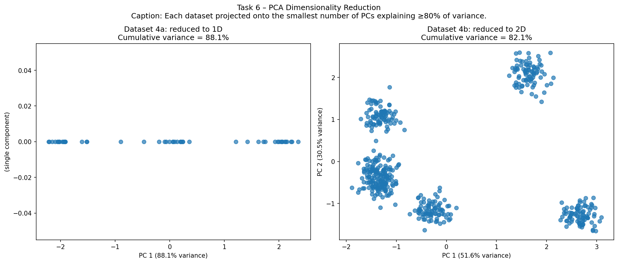
Question 6b: Use PCA to visualize datasets 4a and 4b. Use the smallest dimension that explains at least 80% of total variance.
- Figures of reduced dimension data for datasets 4a and 4b, with the variance each PC explains in axis labels.
- A table of R-squared and MSE for different dimensions in each dataset.
- Which dimension should be selected to explain the most data while still being able to plot the result?
Code
from sklearn.decomposition import PCA
from sklearn.preprocessing import scale as sk_scale
from sklearn.metrics import mean_squared_error as mse_fn

fig, axes = plt.subplots(1, 2, figsize=(14, 6))

for ax, (dname, fname) in zip(axes,
        [('4a','dataset-task-4a.csv'),('4b','dataset-task-4b.csv')]):
    X_pca    = sk_scale(pd.read_csv(fname).values)   # centre + unit variance
    pca_full = PCA().fit(X_pca)
    evr      = pca_full.explained_variance_ratio_
    cumevr   = np.cumsum(evr)
    k_min    = int(np.argmax(cumevr >= 0.80)) + 1     # smallest k ≥ 80%

    # R² / MSE table
    for k_iter in range(1, len(evr)+1):
        pca_k = PCA(n_components=k_iter)
        sc    = pca_k.fit_transform(X_pca)
        r2    = float(np.sum(evr[:k_iter]))
        mse   = mse_fn(X_pca, sc @ pca_k.components_)
        print(f'k={k_iter}  R²={r2:.4f}  MSE={mse:.4f}')

    # Visualise with k_min components
    sc_vis = PCA(n_components=k_min).fit_transform(X_pca)
    if k_min == 1:
        ax.scatter(sc_vis[:,0], np.zeros(len(sc_vis)), alpha=0.7, s=40)
        ax.set_xlabel(f'PC 1 ({evr[0]*100:.1f}% variance)')
    else:
        ax.scatter(sc_vis[:,0], sc_vis[:,1], alpha=0.7, s=40)
        ax.set_xlabel(f'PC 1 ({evr[0]*100:.1f}% variance)')
        ax.set_ylabel(f'PC 2 ({evr[1]*100:.1f}% variance)')
    ax.set_title(f'Dataset {dname}: {k_min}D PCA ({cumevr[k_min-1]*100:.1f}% var.)')
plt.tight_layout();  plt.show()
Why we scale first
sk_scale centres each feature on 0 and scales to unit variance. Without this, PCA would be dominated by whichever feature has the largest numeric range — not necessarily the most informative one. Scaling ensures all features are considered equally by PCA.
Result
R² and MSE tables
Dataset 4a (3 features):
| k | R² (cumulative) | MSE | |
|---|---|---|---|
| 1 | 0.8813 | 0.1187 | ← ≥80% |
| 2 | 0.9753 | 0.0247 | |
| 3 | 1.0000 | 0.0000 | full |
Dataset 4b (5 features):
| k | R² (cumulative) | MSE | |
|---|---|---|---|
| 1 | 0.5163 | 0.4837 | |
| 2 | 0.8210 | 0.1790 | ← ≥80% |
| 3 | 0.9210 | 0.0790 | |
| 4 | 0.9902 | 0.0098 | |
| 5 | 1.0000 | 0.0000 | full |
Which dimension to select?
| Dataset | Min k ≥ 80% var. | Recommended k for plotting | Reason |
|---|---|---|---|
| 4a | k=1 (88.1%) | k=2 (97.5%) | 2D scatter more informative than 1D; cost = +9.4% info at zero plot complexity |
| 4b | k=2 (82.1%) | k=2 (82.1%) | Already ≥80% and directly plotable as 2D scatter |
Dataset 4a: k=1 technically satisfies the 80% threshold (88.1%), but a single-axis plot is much less useful than a 2D scatter. Using k=2 captures 97.5% of variance while producing a standard 2D visualisation — a clear win for minimal extra cost.
Dataset 4b: k=2 exactly satisfies the threshold (82.1%) and directly produces a 2D scatter plot. Adding k=3 gives 92.1% but is no longer directly plotable without further reduction. Therefore k=2 is optimal for both datasets when the goal is to maximise explained variance while remaining plottable.