Code

url_t3 = 'https://raw.githubusercontent.com/MLCourse-LU/Datasets/main/dataset-task-3.csv'
df_t3 = pd.read_csv(url_t3)
X_t3  = df_t3.values
k_t3  = 4

for model_name, clusterer in [
        ('KMeans',   KMeans(n_clusters=4, random_state=42, n_init=10)),
        ('KMedoids', KMedoids(n_clusters=4, random_state=42))]:

    labels = clusterer.fit_predict(X_t3)
    sil_avg = silhouette_score(X_t3, labels)
    sil_vals = silhouette_samples(X_t3, labels)

    fig, (ax1, ax2) = plt.subplots(1, 2, figsize=(16, 6))

    # Left: silhouette bars per cluster
    y_lower = 10
    for i in range(4):
        vals = np.sort(sil_vals[labels == i])
        y_upper = y_lower + len(vals)
        color = cm.nipy_spectral(float(i) / 4)
        ax1.fill_betweenx(np.arange(y_lower, y_upper), 0, vals,
                          facecolor=color, edgecolor=color, alpha=0.7)
        ax1.text(-0.05, y_lower + 0.5*len(vals), str(i))
        y_lower = y_upper + 10
    ax1.axvline(x=sil_avg, color='red', linestyle='--', label=f'Avg={sil_avg:.3f}')
    ax1.set_xlabel('Silhouette coefficient');  ax1.legend()

    # Right: scatter of clusters + centroids
    colors_sc = cm.nipy_spectral(labels.astype(float) / 4)
    ax2.scatter(X_t3[:,0], X_t3[:,1], c=colors_sc, s=30, alpha=0.7, edgecolor='k')
    for i, c in enumerate(clusterer.cluster_centers_):
        ax2.scatter(c[0], c[1], marker=f'${i}$', s=50, edgecolor='k', zorder=6)

    plt.suptitle(f'{model_name} Silhouette (k=4) — avg = {sil_avg:.4f}')
    plt.tight_layout();  plt.show()

How silhouette analysis works

The silhouette coefficient for point i is:

s(i) = (b(i) − a(i)) / max(a(i), b(i))

where a(i) = mean distance to points in same cluster (cohesion) and b(i) = mean distance to points in the nearest other cluster (separation). Score near +1 → well separated; near 0 → on boundary; negative → likely misassigned. The overall average score summarises global cluster quality.

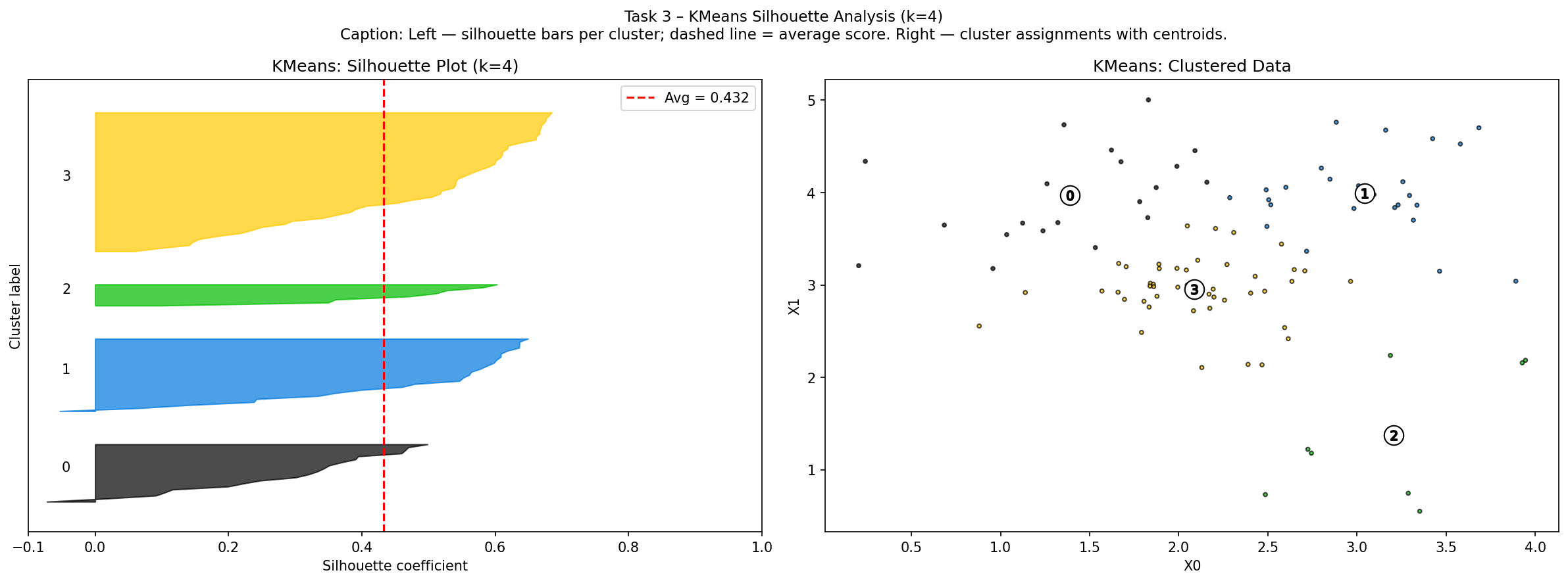
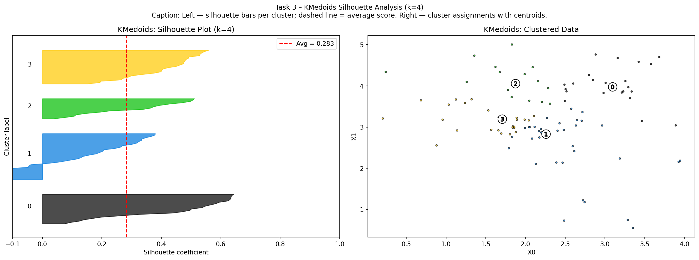
The silhouette plot shows sorted bars for each cluster — wide, positive bars indicate tight, well-separated clusters. The red dashed line marks the average score.

KMeans result (avg silhouette = 0.432)

KMedoids result (avg silhouette = 0.283)

Scores

Model	Average Silhouette Score
KMeans	0.432
KMedoids	0.283

Analysis — why KMeans wins here

Dataset-task-3 contains approximately round, balanced, well-separated blobs — the ideal shape for KMeans. KMeans minimises within-cluster sum of squared distances, which is equivalent to finding the optimal partition for spherical Gaussian clusters. Its centroids sit at the true geometric centre of each cluster.

KMedoids adds the constraint that its centroid must be an actual data point. For clean spherical clusters, this constraint means the medoid is almost never at the true centre — it is slightly off, causing slightly suboptimal cluster boundaries. The robustness advantage of KMedoids (resistance to outliers) is irrelevant when the data is clean.

In short: KMeans is the right tool here because the data matches its assumptions exactly.